Comfortably numb (from deploying too many agents)
Step one of the 12 steps is admitting you have a problem. So here goes:…
Step one of the 12 steps is admitting you have a problem. So here goes:…
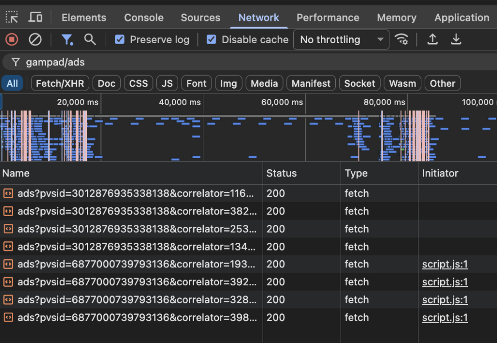
Right now, the reason you got an ad is actually sitting in plain text in…
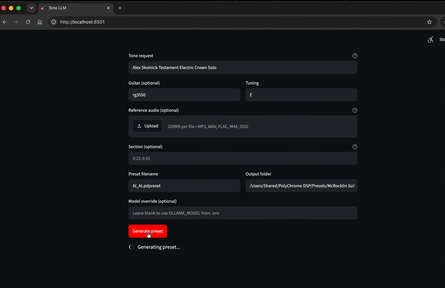
I built tonellm — a Python tool that turns text descriptions into Polychrome DSP amp…
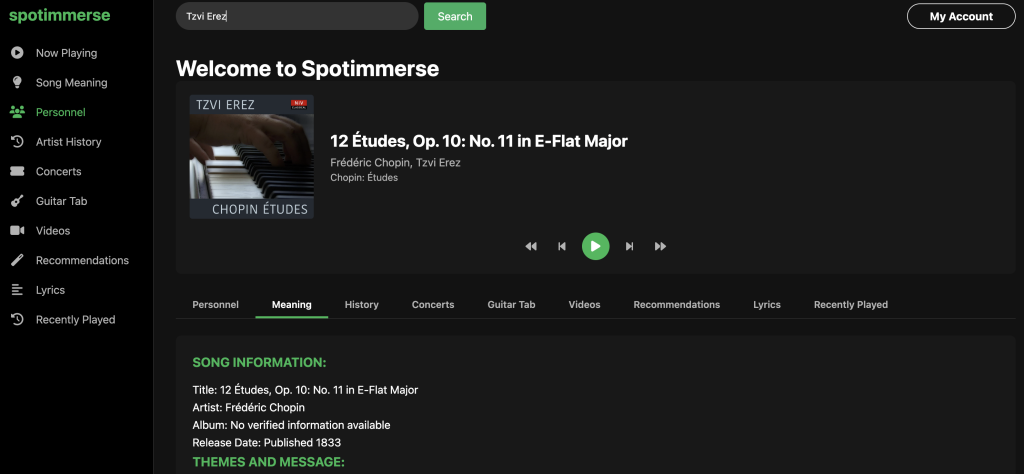
Check out the app here: https://spotimmerse.xyz/ Being addicted to various music genres and being sometimes…
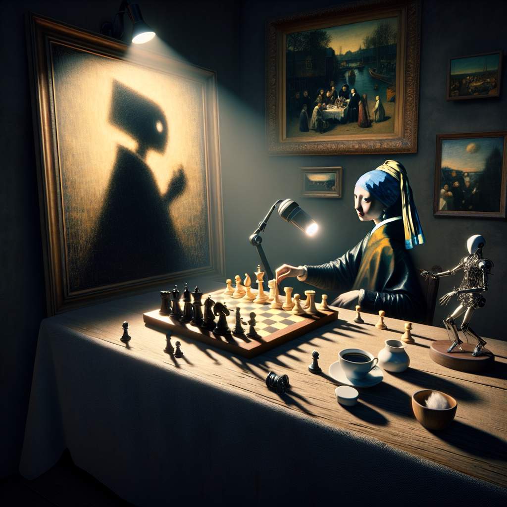
Chrome extension here Chess has always been an intermittent interest of mine even though game…
A friend recently told me keeping up with the latest AI research papers feels like…

The Samsung frame TV has a brilliant Art Mode, that I really enjoy, that adds…

Playing around with the Chat GPT, Bard user interfaces has been fun but I end…

One of my older tracks (trained on a LSTM) to generate a 80s shred inspired…
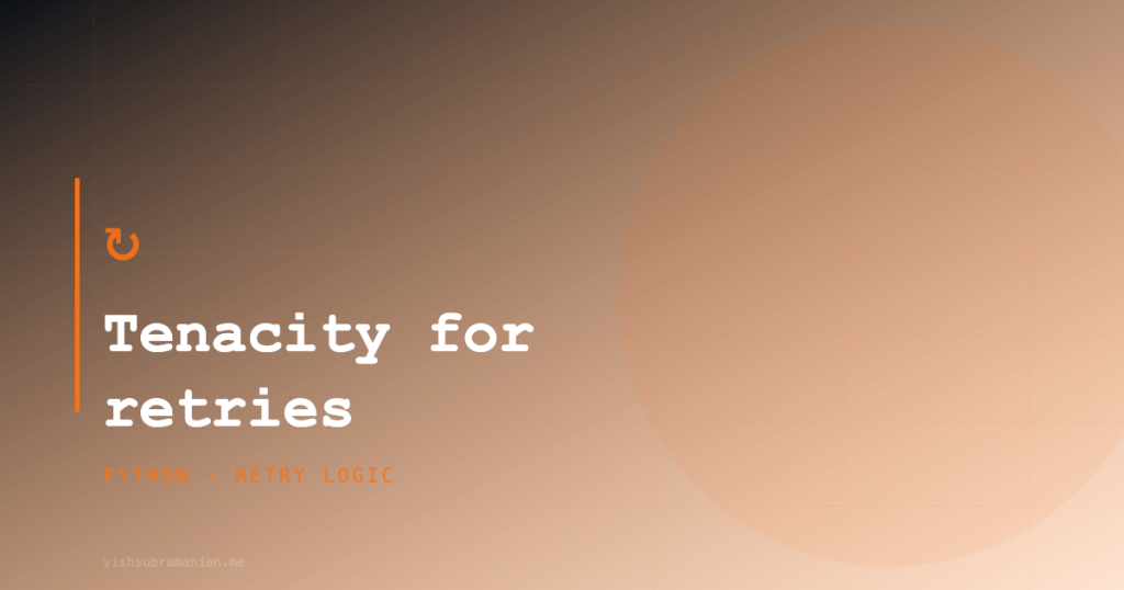
I discovered Tenacity while encountering a bunch of gobbledygook shell and python scripts crunched together…