AdTech Trial – The house always wins
I’ve found the filings on Google’s anti trial case a fascinating primer on adtech best…

I’ve found the filings on Google’s anti trial case a fascinating primer on adtech best…

Chrome extension here Chess has always been an intermittent interest of mine even though game…

The Samsung frame TV has a brilliant Art Mode, that I really enjoy, that adds…
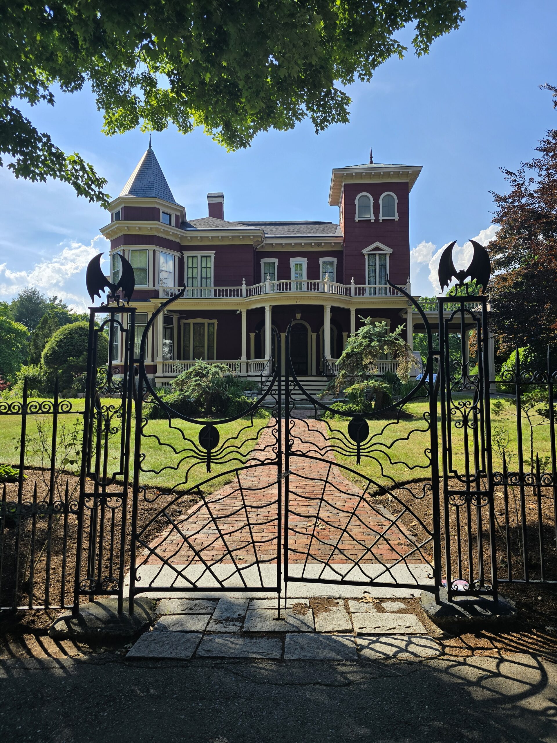
As a massive fan who’s voraciously consumed every Stephen King/Richard Bachman novel written to date, our…

Leading large data engineering teams in the age of LLMs always leads to many existential…

Running large data platforms using 1P, 2P and 3P data involves measuring your AdTech spend…

Playing around with the Chat GPT, Bard user interfaces has been fun but I end…

One of my older tracks (trained on a LSTM) to generate a 80s shred inspired…
CLUSTER now available on streaming platforms. First Principles is a collaboration between Bass Player/ Composer…

With ‘The Last of Us‘ becoming everyone’s favorite live-action adaptation of a video game franchise,…